Pythonで二重振り子のアニメーションを作る

QiitaのPythonタグをなんとなく見ているけれど、機械学習や数学関連の、意識高い投稿が多くて羨ましい。というわけで、今回は意識高く、二重振り子のアニメーションを作ってみる。
…と思って書いていたのだが、もうちょっと調べてから上げようと思っていたら2ヶ月以上経ってしまった。
このままだと永久に公開できない気がしたので、まだちゃんとできていないところがいろいろあるがとりあえず上げておく。
あとで手を加えていく…予定。

環境

• ArchLinux

  • Python 3.6.1
  • pip 9.0.1
  • matplotlib 2.0.0
  • numpy 1.12.1
  • PyQt 5.8.2
  • scipy 0.19.0

• Ubuntu 16.04

  • Python 3.5.2
  • 他は同じ

インストール方法

$ sudo pacman -S python-pip
$ sudo pip install matplotlib scipy numpy pyqt5

Ubuntuなら

$ sudo apt-get install python3-pip
$ pip3 install matplotlib numpy scipy sympy

でいけたはず。Ubuntuだとpipで落とすパッケージは ~/.local/lib/python3.5/site-packages に入れてるっぽいのでsudoが不要なのか。あといちいちpip3とかpython3とか打たないとダメなのが面倒。デフォルトがpython2のため。

matplotlibの設定

ArchLinuxだとそのままでは描画できなかった。

/usr/lib/python3.6/site-packages/matplotlib/mpl-data/matplotlibrc のbackendを qt5aggに変更。

Python で matplotlib を試そうとしたら 'cairo.Context' ってナニソレ - Qiita参照。

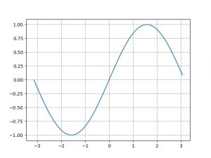
matplotlibのテスト: sin

sin曲線を描画してみる。

import numpy as np
import matplotlib.pyplot as plt

PI = np.pi
x = np.arange(-PI, PI, 0.1)
y = np.sin(x)
plt.grid()
plt.plot(x, y)
plt.show()

numpyパッケージをnpという名前でimportしている。 numpy.arange (arrangeではない)はNumPy配列を返し、 numpy.sin は配列の各要素に対してsinの値を返す。

• NumPy配列
  numpy.ndarray のことをNumPy配列と呼ぶらしい。これはN-Dimension Arrayだからndarrayのよう。
  面白いのは y = np.sin(x) の x も y もNumPy配列になっていること。つまりxの各要素のsinを取ったものがy。
  なおPythonでは普通の配列はlist。型は type でわかる。

  >>> import numpy as np
  >>> a = np.array([1, 2, 3])
  >>> a
  array([1, 2, 3])
  >>> type(a)
  <class 'numpy.ndarray'>
  >>> b = [1, 2, 3]
  >>> b
  [1, 2, 3]
  >>> type(b)
  <class 'list'>
  

• numpy.arange([start, ]stop[, step])
  startからstopをstepずつ増やしたNumPy配列を返す。numpy.arange — NumPy v1.12 Manual参照。

  >>> import numpy as np
  >>> np.arange(5)
  array([0, 1, 2, 3, 4])
  >>> np.arange(5, 9)
  array([5, 6, 7, 8])
  >>> np.arange(5, 9, 2)
  array([5, 7])
  

• pyplot.grid()
  グリッドを描く。pyplot — Matplotlib 2.0.2 documentation参照。
  色とか線の形などを変えるときは以下のようにする。

  plt.grid(color='r', linestyle='dotted', linewidth=1)
  

• pyplot.plot()
  グラフを描く。pyplot — Matplotlib 2.0.2 documentation参照。
  色とか線の形などを変えるときはgridと同様。

  plt.plot(x, y, color='r', linestyle='dotted', linewidth=3)
  

  これと同じことを略記して

  plt.plot(x, y, 'r--', linewidth=3)
  

  とも書ける。

• numpy.sin, numpy.cos, numpy.pi
  はじめに

  from numpy import sin, cos, pi
  

  と書いておけば、いちいち np.sin とか書かなくても sin だけで書ける。

比率の固定

上で描画したsin曲線のグラフは、ウィンドウのサイズを変えると縦長になったり横長になったりして比率が変わる。それを固定化する。 図の中にもう一つ図(サブプロット)を入れて、サブプロットにいろいろ設定して描画する感じ。

import numpy as np
import matplotlib.pyplot as plt

PI = np.pi
x = np.arange(-PI, PI, 0.1)
y = np.sin(x)

fig = plt.figure()
ax = fig.add_subplot(111, aspect='equal', autoscale_on=False, xlim=(-PI, PI), ylim=(-PI, PI))
ax.grid()

plt.plot(x, y)
plt.show()

• figure.Figure.add_subplot
  figure — Matplotlib 2.0.2 documentation参照。
  これを使うと複数のグラフを並べて描ける。
  最初の'111'というのはグラフの位置指定。たとえばこれが'234'なら、ウィンドウを縦2横3に分割して、その(左上から右、そして下に数えて)4番目を使うということ。
  以下のような感じ。

  import numpy as np
  import matplotlib.pyplot as plt
  
  PI = np.pi
  
  fig = plt.figure()
  
  ax = fig.add_subplot(234, aspect='equal', autoscale_on=False, xlim=(-PI, PI), ylim=(-PI, PI))
  x1 = np.arange(-PI, PI, 0.1)
  y1 = np.sin(x1)
  ax.grid()
  plt.plot(x1, y1)
  
  ax = fig.add_subplot(232, aspect='equal', autoscale_on=False, xlim=(-PI, PI), ylim=(-PI, PI))
  x2 = np.arange(-PI, PI, 0.1)
  y2 = np.cos(x2)
  ax.grid(color='b', linestyle='dotted', linewidth=0.1)
  plt.plot(x2, y2, 'r--')
  
  plt.show()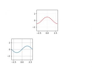
  

  

微分方程式の数値計算: 自由落下

dy/dt = f(t, y)という形の常微分方程式を解くのはscipy.integrate.odeintでできる。scipy.integrate.odeint — SciPy v0.18.1 Reference Guide 参照。
FORTRANのodepackにあるlsodaという関数(？)を使って数値計算しているそう。

たとえば自由落下はy軸を鉛直上向きに取って $\cfrac{d^{2}y}{dt^2} = -g$ なので、これを1階に分解して $$\left\{ \begin{array}{l} \cfrac{dy}{dt} = v\\ \cfrac{dv}{dt} = -g \end{array} \right.$$

import numpy as np
from scipy.integrate import odeint

def ode(f, t):
    y, v = f
    dfdt = [v, -G]
    return dfdt

G  = 9.8        # [m/s^2] gravitational acceleration
V0 = 0          # [m/s]   initial velocity
DURATION = 10   # [s] duration time
INTERVAL = 1    # [s] interval time

f0 = [0, V0]    # [y, v] at t = 0
t = np.linspace(0, DURATION, DURATION + INTERVAL)

sol = odeint(ode, f0, t)
print(sol)

f0には[y, v]の初期値を入れている。ode(f, t)はただの連立微分方程式で、ここに上に書いた自由落下の式を入れている。

結果は以下。 [[y, v] at t = 0, [y, v] at t = 1, ..., [y, v] at t = 10] ってこと。

[[   0.     0. ]
 [  -4.9   -9.8]
 [ -19.6  -19.6]
 [ -44.1  -29.4]
 [ -78.4  -39.2]
 [-122.5  -49. ]
 [-176.4  -58.8]
 [-240.1  -68.6]
 [-313.6  -78.4]
 [-396.9  -88.2]
 [-490.   -98. ]]

• numpy.linspace(start, stop, num)
  startからstopまでをnum等分した配列を返す。 numpy.arange とよく似てる。こんなメソッドもあるということで使ってみた。
  numpy.linspace — NumPy v1.12 Manualを参照。

  >>> import numpy as np
  >>> np.linspace(1, 3, 5)
  array([ 1. ,  1.5,  2. ,  2.5,  3. ])
  

• y, v = f
  Pythonではこんな書き方ができるらしい。いらない要素は _ に入れればいいっぽい。

  >>> x = [1, 2, 3]
  >>> a, _, c = x
  >>> a
  1
  >>> c
  3
  

数値計算の結果をアニメーションにする

上の結果をアニメーションにする。自由落下だと退屈なので、ちょっと上向きに放ってみる。
なお、最後の2行はアニメーションをmp4/gifで保存するためのもの。いらなければコメントアウトしていい。

import matplotlib.pyplot as plt
import numpy as np
from matplotlib.animation import FuncAnimation
from scipy.integrate import odeint

def ode(f, t):
    y, v = f
    dfdt = [v, -G]
    return dfdt

G  = 9.8        # [m/s^2] gravitational acceleration
V0 = 20         # [m/s]   initial velocity
DURATION = 10   # [s] duration time
INTERVAL = 0.1  # [s] interval time

f0 = [0, V0]    # [y, v] at t = 0
t = np.arange(0, DURATION + INTERVAL, INTERVAL)

sol = odeint(ode, f0, t)



fig = plt.figure()
ax = fig.add_subplot(111, aspect='equal', autoscale_on=False, xlim=(-100, 100), ylim=(-500, 100))
ax.grid()

ball, = plt.plot([], [], 'ro', animated=True)

def init():
    return ball,

def update(y):
    ball.set_data(0, y)
    return ball,

FRAME_INTERVAL = 1000 * INTERVAL # [msec] interval between frames
FPS = 1000/FRAME_INTERVAL # frames per second

ani = FuncAnimation(fig, update, frames=sol[:, 0],
                    init_func=init, blit=True, interval=FRAME_INTERVAL, repeat=True)
plt.show()
ani.save('fall.mp4', fps=FPS, extra_args=['-vcodec', 'libx264'])
ani.save('fall.gif', writer='imagemagick', fps=FPS)

• set_data()
  lines — Matplotlib 2.0.2 documentation参照。
  座標を指定すればその通りに描画される。

• ball, = plt.plot([], [], 'ro', animated=True)
  この , はどう見ても間違ってると思ったのだが…。 これは plt.plot([], [], 'ro', animated=True) がlist(要素数1)で、 ball にそのlistの中身を入れるためにやるよう。 animation example code: simple_anim.py — Matplotlib 2.0.2 documentationでもやってるので同じようにやった。
  plt.plot([], [], 'ro', animated=True) で2つ[]を入れているのは自信なし。

  >>> a, = [999]
  >>> a
  999
  

• sol[:, 0]
  NumPy多重配列のslice。solは多重配列だが、要素の配列の0番目を集めた配列ということ。
  Python (numpy) で出てくるコロン,カンマ [:,]参照。

  >>> import numpy as np
  >>> a = np.array([[1, 2, 3], [4, 5, 6], [7, 8, 9]])
  >>> a
  array([[1, 2, 3],
         [4, 5, 6],
         [7, 8, 9]])
  >>> a[:, 0]
  array([1, 4, 7])
  

単振り子のアニメーション

二重振り子ではどうせ解析力学を使うので、これも同じようにやってやる。
Lagrangianは $$L = \cfrac{1}{2}ml^2\dot{\theta}^2 + mgl\cos\theta$$ なのでEuler-Lagrange eq.は $$\ddot{\theta} = - \cfrac{g}{l} \sin\theta$$ これを数値計算するために1階に分解してやると $$\left\{ \begin{array}{l} \cfrac{d\theta}{dt} = \dot{\theta}\\ \cfrac{d\dot{\theta}}{dt} = -\cfrac{g}{l}\sin\theta \end{array} \right.$$ のような形になる。あとは落下のときと同様に描画してやればいい。
経過時間を表示するようにしてみた。

import matplotlib.pyplot as plt
import numpy as np
from numpy import sin, cos, pi
from matplotlib.animation import FuncAnimation
from scipy.integrate import odeint

def ode(f, t):
    theta, dtheta = f
    dfdt = [dtheta, -(G/L) * sin(theta)]
    return dfdt

G  = 9.8         # [m/s^2] gravitational acceleration
THETA0 = pi/4    # [rad]   initial angle
V0 = 1           # [m/s]   initial velocity
L = 1            # [m]     length of the pendulum
DURATION = 10    # [s]     duration time
INTERVAL = 0.05  # [s]     interval time

f0 = [THETA0, V0/L]    # [theta, v] at t = 0
t = np.arange(0, DURATION + INTERVAL, INTERVAL)

sol = odeint(ode, f0, t)

fig = plt.figure()
ax = fig.add_subplot(111, aspect='equal', autoscale_on=False, xlim=(-L, L), ylim=(-L, L))
ax.grid()

theta = sol[:, 0]
x = L * sin(theta)
y = - L * cos(theta)
line, = plt.plot([], [], 'ro-', animated = True)

time_template = 'time = %.1fs'
time_text = ax.text(0.05, 0.9, '', transform=ax.transAxes)

def init():
    time_text.set_text('')
    return line, time_text

def update(i):
    next_x = [0, x[i]]
    next_y = [0, y[i]]
    line.set_data(next_x, next_y)

    time_text.set_text(time_template % (i*INTERVAL))
    return line, time_text

FRAME_INTERVAL = 1000 * INTERVAL # [msec] interval between frames
FPS = 1000/FRAME_INTERVAL # frames per second

ani = FuncAnimation(fig, update, frames=np.arange(0, len(t)),
                    interval=FRAME_INTERVAL, init_func=init, blit=True)
plt.show()
ani.save('single_pendulum.mp4', fps=FPS, extra_args=['-vcodec', 'libx264'])
ani.save('single_pendulum.gif', writer='imagemagick', fps=FPS)

二重振り子のアニメーション

数式を書いてるが、正しさは一切責任持たない。typoあると思う。
角度や長さなどの記号は二重振り子 - Wikipediaと同じ。

Lagrangianは $$L = \cfrac{1}{2} (m_{1} + m_{2}) l_{1}^{2} \dot{\theta_{1}}^{2} + \cfrac{1}{2} m_{2} l_{2}^{2} \dot{\theta_{2}}^{2} + m_{2} l_{1} l_{2} \dot{\theta_{1}} \dot{\theta_{2}} \cos(\theta_{2} - \theta_{1}) + (m_{1} + m_{2}) gl_{1}\cos\theta_{1} + m_{2}gl_{2}\cos\theta_{2}$$

あとはE-L eq.を求めて、それを1階微分だけの連立微分方程式に分解すればいい。
面倒な計算をすると $$\left\{ \begin{array}{l} \cfrac{d\theta_{1}}{dt} = \dot{\theta_{1}}\\ \cfrac{d\theta_{2}}{dt} = \dot{\theta_{2}}\\ \cfrac{d\dot{\theta_{1}}}{dt} = \cfrac{1}{l_{1}l_{2} \left( m_{1} + m_{2} \sin^2 (\theta_{2} - \theta_{1})\right)} l_{2} \left( m_{2} g \sin\theta_{2} \cos(\theta_{2} - \theta_{1}) + m_{2} l_{1} \dot{\theta_{1}}^2 \sin(\theta_{2} - \theta_{1}) \cos(\theta_{2} - \theta_{1}) + m_{2} l_{2} \dot{\theta_{2}}^2 \sin(\theta_{2} - \theta_{1}) - (m_{1} + m_{2}) g \sin\theta_{1}\right)\\ \cfrac{d\dot{\theta_{2}}}{dt} = \cfrac{1}{l_{1}l_{2} \left( m_{1} + m_{2} \sin^2 (\theta_{2} - \theta_{1})\right)} l_{1} \left( -(m_{1} + m_{2}) l_{1} \dot{\theta_{1}}^2 \sin(\theta_{2} - \theta_{1}) - (m_{1} + m_{2}) g \sin\theta_{2} - m_{2}l_{2}\dot{\theta_{2}}^2\sin(\theta_{2} - \theta_{1}) \cos(\theta_{2} - \theta_{1}) + (m_{1} + m_{2})g\sin\theta_{1} \cos(\theta_{2} - \theta_{1}) \right) \end{array} \right.$$ を(たぶん)得る。

あとは同じようにやればいい。
単振り子と違うのは、質点が2個あること。これは単振り子のときに $f = [\theta, \dot{\theta}]$ としていたのを $f = [\theta_{1}, \dot{\theta_{1}}, \theta_{2}, \dot{\theta_{2}}]$ とすればいい。

from numpy import sin, cos, pi
import matplotlib.pyplot as plt
from matplotlib.animation import FuncAnimation
import numpy as np
from scipy.integrate import odeint

def ode(f, t):
    theta1, dtheta1, theta2, dtheta2 = f
    dtheta1dt = (M2 * G * sin(theta2) * cos(theta2 - theta1)
            + M2 * L1 * (dtheta1 ** 2) * sin(theta2 - theta1) * cos(theta2 - theta1)
            + M2 * L2 * (dtheta2 ** 2) * sin(theta2 - theta1)
            - (M1 + M2) * G * sin(theta1)) / (M1 * L1 + M2 * L1 * (sin(theta2 - theta1) ** 2))
    dtheta2dt = (-(M1 + M2) * L1 * (dtheta1 ** 2) * sin(theta2 - theta1)
            - (M1 + M2) * G * sin(theta2)
            - M2 * L2 * (dtheta2 ** 2) * sin(theta2 - theta1) * cos(theta2 - theta1)
            + (M1 + M2) * G * sin(theta1) * cos(theta2 - theta1)) / (M1 * L2 + M2 * L2 * (sin(theta2 - theta1) ** 2))
    return [dtheta1, dtheta1dt, dtheta2, dtheta2dt]

G  = 9.8            # [m/s^2]  gravitational acceleration
THETA1_0 =  pi      # [radian] initial theta
THETA2_0 =  pi/6    # [radian] initial theta
V1_0 = 0            # [m/s]    initial velocity
V2_0 = 0            # [m/s]    initial velocity
L1 =  1             # [m]      length of pendulum
L2 =  1             # [m]      length of pendulum
M1 =  1             # [kg]     mass
M2 =  1             # [kg]     mass
DURATION = 10       # [s]      duration time
INTERVAL = 0.05     # [s]      interval time

f_0 = [THETA1_0, V1_0/L1, THETA2_0, V2_0/L2]
t = np.arange(0, DURATION + INTERVAL, INTERVAL)

sol = odeint(ode, f_0, t)
theta1, theta2 = sol[:, 0], sol[:, 2]

x1 = L1 * sin(theta1)
y1 = - L1 * cos(theta1)
x2 = x1 + L2 * sin(theta2)
y2 = y1 - L2 * cos(theta2)

fig = plt.figure()
ax = fig.add_subplot(111, aspect='equal', autoscale_on=False, xlim = [-L1 - L2, L1 + L2], ylim = [-L1 - L2, L1 + L2])
ax.grid()

line, = plt.plot([], [], 'ro-', animated = True)

time_template = 'time = %.1fs'
time_text = ax.text(0.05, 0.9, '', transform=ax.transAxes)

def init():
    time_text.set_text('')
    return line, time_text

def update(i):
    next_x = [0, x1[i], x2[i]]
    next_y = [0, y1[i], y2[i]]
    line.set_data(next_x, next_y)

    time_text.set_text(time_template % (i * INTEtrueVAL))
    return line, time_text

FRAME_INTERVAL = 1000 * INTERVAL # [msec] interval time between frames
FPS = 1000/FRAME_INTERVAL        # frames per second
ani = FuncAnimation(fig, update, frames=np.arange(0, len(t)),
                    interval=FRAME_INTERVAL, init_func=init, blit=True)

plt.show()
ani.save('double_pendulum.mp4', fps=FPS, extra_args=['-vcodec', 'libx264'])
ani.save('double_pendulum.gif', writer='imagemagick', fps=FPS)

感想

Qiitaとかに数式ゴリゴリ書いている人たちの情熱はすごい。もう数式とか書きたくない。
あと複雑系はけっこう好きなので、こうやって数値計算できるのは楽しい。

参考

• 二重振り子について
  • 二重振り子 - Wikipedia
• ArchLinuxでの描画について
  • Python で matplotlib を試そうとしたら 'cairo.Context' ってナニソレ - Qiita
• odeint
  • scipy.integrate.odeint — SciPy v0.18.1 Reference Guide
  • ODEPACK
• add_subplot
  • figure — Matplotlib 2.0.2 documentation
  • python - In Matplotlib, what does the argument mean in fig.add_subplot(111)? - Stack Overflow
• FuncAnimation
  • matplotlib でアニメーションを作る - Qiita
  • animation module — Matplotlib 2.0.0 documentation
  • matplotlib.animation.FuncAnimation — Matplotlib 2.0.0 documentation
  • animation example code: simple_anim.py — Matplotlib 2.0.2 documentation
• pyplot
  • pyplot — Matplotlib 2.0.2 documentation
• NumPy
  • numpy.arange — NumPy v1.12 Manual
  • numpy.linspace — NumPy v1.12 Manual
  • NumPy 配列の基礎 — 機械学習の Python との出会い
  • numpy.ndarray — NumPy v1.12 Manual